Benchmarking Cookbook • gseries

Description of the steps of a typical benchmarking project with G-Series (R package gseries).

Other useful resources related to the time series benchmarking problem discussed here and solved using the G-Series benchmarking functions (benchmarking() and stock_benchmarking()), in ascending order of technical complexity:

Fortier and Quenneville (2007), in References for function benchmarking(), for an overview of the time series benchmarking methodology implemented in G-Series including detailed examples. This document is available in GCdocs for Statistics Canada employees (search for “ICES2007_Fortier.pdf” in GCDocs).
Course 0436, “Theory and Application of Benchmarking”, in References for function benchmarking() and stock_benchmarking(). Visit the Course 0436 web page (Statistics Canada general public website) for more details.
Dagum and Cholette (2006), in References for function benchmarking(), for a complete technical discussion and presentation of time series benchmarking problems and their solution.

1. Prepare the input data

The first step usually involves converting “ts” or “mts” objects (stats package) into the proper format for the G-Series benchmarking functions with the following two utility functions;

ts_to_tsDF() for the indicator series
ts_to_bmkDF() for the benchmarks

It is possible to benchmark multiple series in a single call to the benchmarking functions. This can be done by specifying the appropriate list of data frame variables with arguments var and with, which can be cumbersome and make your code look cluttered. A more convenient option to achieve the same result would be to use the allCols argument. However, these two alternatives have important limitations as they both require that all the indicator series are of the same length (same number of periods) and have the same set (number) of benchmarks. The values of the benchmarks can obviously differ for each indicator series, but their coverage must be the same.

A more flexible approach, which doesn’t suffer from the aforementioned limitations, is to use the BY-group mode (argument by) of the benchmarking functions after having converted the input data frames into stacked (tall) versions with the following utility functions:

stack_tsDF() for the indicator series
stack_bmkDF() for the benchmarks

Stacked versions of the data frames use only two variables to specify information about the different indicator series or benchmarks: one variable for the identifiers and another for the values. A stacked data frame therefore contains more rows but fewer variables (columns) than a non-stacked data frame as the time series are stacked on top of each other instead of being layed out side by side. BY-group processing with stacked data frames is the recommended approach to benchmark several series in a single benchmarking function call, unless the number of series to benchmark is extremely large and processing time is a really important issue (processing multiple time series with arguments var or allCols should be slightly faster than the BY-group approach with argument by).

2. Run benchmarking

The number of calls to the benchmarking functions depends on the values of arguments rho, lambda, biasOption and bias (plus low_freq_periodicity, n_low_freq_proj and proj_knots_rho_bd for function stock_benchmarking()). One call is necessary for each distinct combination of these argument values. In practice, however, only argument lambda will usually require distinct values to process the entire set of series: lambda = 1 for proportional benchmarking and lambda = 0 for additive benchmarking. Two calls to the benchmarking functions are therefore often enough.

When more than one call is required, the input indicator series and benchmarks data frames need to be split into distinct data frames: one for each call with the relevant set of indicator series and benchmarks. Alternatively, one can add one or several columns to the stacked versions of the input data frames in order to identify (and extract) the indicator series and benchmarks of each call.

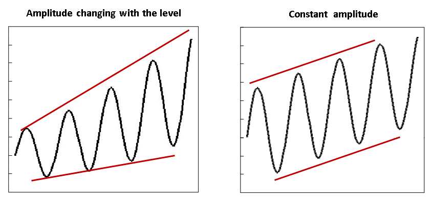
Note on proportional and additive benchmarking
Proportional benchmarking (\lambda \ne 0) is normally used when the main focus is the preservation of period-to-period ratios (relative differences) and additive benchmarking (\lambda = 0) for the preservation of period-to-period differences. Focusing on period-to-period ratios is usually preferable for time series for which the amplitude (e.g., seasonal and irregular components) changes with the level of the series. On the other hand, if the amplitude of the series stays relatively constant regardless of the level of the series, then looking at period-to-period differences is appropriate.

Series Amplitude

The most common pitfall would likely be using an additive benchmarking approach when changes in the amplitude of the indicator series are important and follow the level (the amplitude increases/decreases with the level). The main advantage of additive benchmarking is that it works (returns a solution) in all contexts while proportional benchmarking will fail in some particular cases (e.g., nonzero benchmark with zero indicator series values for all periods covered by the benchmark). Proportional benchmarking with \rho < 1 (regression-based benchmarking) generally works well in practice (provides reasonable solutions) with problems involving values of zero for the indicator series and/or the benchmarks. Some people may actually appreciate (find appealing) the fact that values of zero in the initial indicator series always remain zero in proportionally benchmarked series, which is not the case for additively benchmarked series. As for proportional benchmarking with \rho = 1 (Denton benchmarking), the indicator series must be strictly positive. However, one could try using argument constant in order to add a (relatively small) temporary constant to the input data and solve cases that involve values of zero in the indicator series. In practice, note that proportional Denton benchmarking could also be approximated with the regression-based approach by using a \rho value that is smaller than, but very close to, 1.0 (e.g., \rho = 0.999). Finally, although proportional benchmarking (\lambda \ne 0, \forall \rho) is not allowed by default in presence of negative values, this behaviour can be modified with argument negInput_option. In any case, one should closely monitor proportionally benchmarked series involving negative values or values of zero (or almost zero) where ratios may be undefined, unstable or difficult to interpret. The resulting proportionally benchmarked data should be carefully analyzed and validated in such cases to make sure they correspond to reasonable, interpretable solutions.

3. Validate the results

Any warning and error message generated by the benchmarking functions should be investigated in order to fix the corresponding issue(s). Once clean executions of the benchmarking functions (free of warning and error messages) are obtained, one should validate the resulting benchmarked series data. Utility function plot_graphTable() generates useful graphics to perform such a task.

Examples of things to look for in the benchmarking results:

Inadequate projected benchmarking adjustments. The benchmarking solution for periods not covered by a benchmark at the end of the series is driven by parameter \rho (argument rho) and the specified bias adjustment (arguments biasOptionand bias). Bias adjustment is generally recommended when the levels of the benchmarks and the indicator series are systematically different (e.g., benchmarks always, or almost always, larger than the indicator series or vice versa). Not correcting for an (important) bias may result in poor results for the benchmarked series for periods not covered by a benchmark (poor projected benchmarking adjustments), which may then lead to large revisions as new benchmarks become available in the future. Correcting for the bias should help in such cases. An exception is Denton benchmarking (\rho = 1) where bias adjustment has no impact on the benchmarking solution. Changing the value of parameter \rho, which dictates the speed at which the projected adjustments converge to the bias for periods not covered by a benchmark, may also improve the situation. The smaller the value of \rho the faster the convergence, with immediate convergence when \rho = 0 and no convergence at all (the adjustment of the last period covered by a benchmark is repeated) when \rho = 1 (Denton benchmarking). A general recommendation that works reasonably well in most cases is to adjust with the estimated average bias (biasOption = 3 and bias = NA) and use \rho = 0.9 for monthly indicators and \rho = 0.9^3 = 0.729 for quarterly indicators. Specifying a user-defined bias (argument bias) may be relevant if the discrepancies between the two sources of data have changed over time (e.g., specifying a value more representative of the recent bias). An alternative would be to use explicit forecasts for the benchmarks at the end of the series instead of relying on the implicit projected benchmarks associated to the bias adjustment and parameter \rho. For example, available auxiliary information could be used to generate explicit benchmarks and (if the projections are good) reduce revisions once the true benchmark values are known. The first two benchmarking graphs (Original Scale Plot and Adjustment Scale Plot) of function plot_graphTable() should help identify potential issues with the projections.
Inadequate autoregressive parameter \rho (argument rho). The goal of benchmarking usually is to preserve the period to period movements of the indicator series, to which correspond values of \rho relatively close to 1 and smooth benchmarking adjustments. This being said, some particular cases may warrant small values of \rho corresponding to less smooth adjustments and reduced movement preservation. The 2^nd benchmarking graph (Adjustment Scale Plot) of function plot_graphTable() shows the benchmarking adjustments and can therefore be used to assess the smoothness of the adjustments and modify, if necessary, the value of parameter \rho. The corresponding degree of movement preservation is illustrated by the 3^rd and 4^th benchmarking graphs (Growth Rates Plot and Table) of function plot_graphTable(). Note that the benchmarking adjustments can also be plotted using utility function plot_benchAdj().
Inadequate adjustment model parameter \lambda (argument lambda). Additive benchmarking is implemented when \lambda = 0 and proportional benchmarking otherwise (when \lambda \ne 0). Choosing the ideal adjustment model may not necessarily be obvious. Refer to the Note on proportional and additive benchmarking above for some insights. Trying both an additive and a proportional benchmarking approach and comparing the benchmarking graphics may help choose the benchmarking adjustment model. For example, the approach that generates a more natural looking benchmarked series in the Original Scale Plot (1^st graph), smoother benchmarking adjustments in the Adjustment Scale Plot (2^nd graph) and better movement preservation in the Growth Rates Plot and Table (3^rd and 4^th graphs) should be favoured. Looking at the benchmarking graphics of function plot_graphTable() should also help identify problematic solutions that may require a change of adjustment model. For example, problematic cases of proportional benchmarking problems with negative values (see argument negInput_option) or values of zero or almost zero for the benchmarks or the indicator series would most likely generate odd looking benchmarked series in the Original Scale Plot, extreme or non-smooth adjustments in the Adjustment Scale Plot or poor movement preservation in the Growth Rates Plot and Table. An additive benchmarking approach may be a better alternative in such cases.

Systematically looking at all the graphics may not necessarily be feasible in practice for large benchmarking projects involving many series. A (crude) classification analysis of the benchmarking functions’ graphTable output data frame (the input of function plot_graphTable()) may help identify cases requiring further investigation and a closer look at the benchmarking graphics.

Note on stock series
Benchmarking stock series with the benchmarking() function generates non smooth adjustments (kinks) around each benchmark, regardless of the values of \rho and \lambda. This is due to the nature of the benchmarks, i.e., discrete values covering a single period (anchor points). Function stock_benchmarking(), specifically aimed at benchmarking stock series, usually provides better results (i.e., improved movement preservation and smoother adjustments). Function plot_benchAdj() is especially useful to compare (overlay) the adjustments of stock series generated by functions benchmarking() and stock_benchmarking(). See Details for the stock_benchmarking() function for more information on the benchmarking of stock series.

4. Process the benchmarked data

The final step usually involves converting the output benchmarked series data (benchmarking functions’ series output data frame) into “ts” (or “mts”) objects with utility function tsDF_to_ts(). When BY-group processing (by argument) is used, one would first need to unstack the benchmarked series data using utility function unstack_tsDF() before calling the tsDF_to_ts() function.

Nonbinding benchmarks
Although benchmarking problems involving nonbinding benchmarks (benchmarking alterability coefficients greater than 0) are relatively rare in practice, it’s important to remember that the benchmarking functions’ output benchmarks data frame always contains the original (unmodified) benchmarks provided as input. In such cases, the modified nonbinding benchmarks would be recovered (calculated) from the output series data frame instead. For example, flows resulting from a benchmarking() call can be aggregated using function stats::aggregate.ts() after having converted the series output data frame into a “ts” object with utility function tsDF_to_ts().