Plot benchmarking adjustments

Plot benchmarking adjustments for a single series in the current (active) graphics device. Up to three types of adjustments can be overlayed in the same plot:

• Adjustments generated by function benchmarking()

• Adjustments generated by function stock_benchmarking()

• Cubic spline associated to adjustments generated by function stock_benchmarking()

These plots can be useful to assess the quality of the benchmarking results and compare the adjustments generated by both benchmarking functions (benchmarking() and stock_benchmarking()) for stock series.

Usage

plot_benchAdj(
  PB_graphTable = NULL,
  SB_graphTable = NULL,
  SB_splineKnots = NULL,
  legendPos = "bottomright"
)

Arguments

PB_graphTable

(optional)

Data frame (object of class "data.frame") corresponding to the benchmarking() (PB for "Proc Benchmarking" approach) function output graphTable data frame. Specify NULL not to include the benchmarking() adjustments in the plot.

Default value is PB_graphTable = NULL.

SB_graphTable

(optional)

Data frame (object of class "data.frame") corresponding to the stock_benchmarking() (SB) function output graphTable data frame. Specify NULL not to include the stock_benchmarking() adjustments in the plot.

Default value is SB_graphTable = NULL.

SB_splineKnots

(optional)

Data frame (object of class "data.frame") corresponding to the stock_benchmarking() (SB) function output splineKnots data frame. Specify NULL not to include the stock_benchmarking() cubic spline in the plot.

Default value is SB_splineKnots = NULL.

legendPos

(optional)

String (keyword) specifying the location of the legend in the plot. See the description of argument x in the documentation of graphics::legend() for the list of valid keywords. Specify NULL not to include a legend in the plot.

Default value is legendPos = "bottomright".

Value

This function returns nothing (invisible(NULL)).

Details

graphTable data frame (arguments PB_graphTable and SB_graphTable) variables used in the plot:

• t for the x-axis values (t)

• benchmarkedSubAnnualRatio for the Stock Bench. (SB) and Proc Bench. (PB) lines

• bias for the Bias line (when \(\rho < 1\))

splineKnots data frame (argument SB_splineKnots) variables used in the plot:

• x for the x-axis values (t)

• y for the Cubic spline line and the Extra knot and Original knot points

• extraKnot for the type of knot (Extra knot vs. Original knot)

See section Value of benchmarking() and stock_benchmarking() for more details on these data frames.

See also

plot_graphTable() bench_graphs benchmarking() stock_benchmarking()

Examples

#######
# Preliminary setup

# Quarterly stocks (same annual pattern repeated for 7 years)
qtr_ts <- ts(rep(c(85, 95, 125, 95), 7), start = c(2013, 1), frequency = 4)

# End-of-year stocks
ann_ts <- ts(c(135, 125, 155, 145, 165), start = 2013, frequency = 1)

# Proportional benchmarking
# ... with `benchmarking()` ("Proc Benchmarking" approach)
out_PB <- benchmarking(
  ts_to_tsDF(qtr_ts), 
  ts_to_bmkDF(ann_ts, discrete_flag = TRUE, alignment = "e", ind_frequency = 4),
  rho = 0.729, lambda = 1, biasOption = 3,
  quiet = TRUE)
# ... with `stock_benchmarking()`
out_SB <- stock_benchmarking(
  ts_to_tsDF(qtr_ts), 
  ts_to_bmkDF(ann_ts, discrete_flag = TRUE, alignment = "e", ind_frequency = 4),
  rho = 0.729, lambda = 1, biasOption = 3,
  quiet = TRUE)


#######
# Plot the benchmarking adjustments

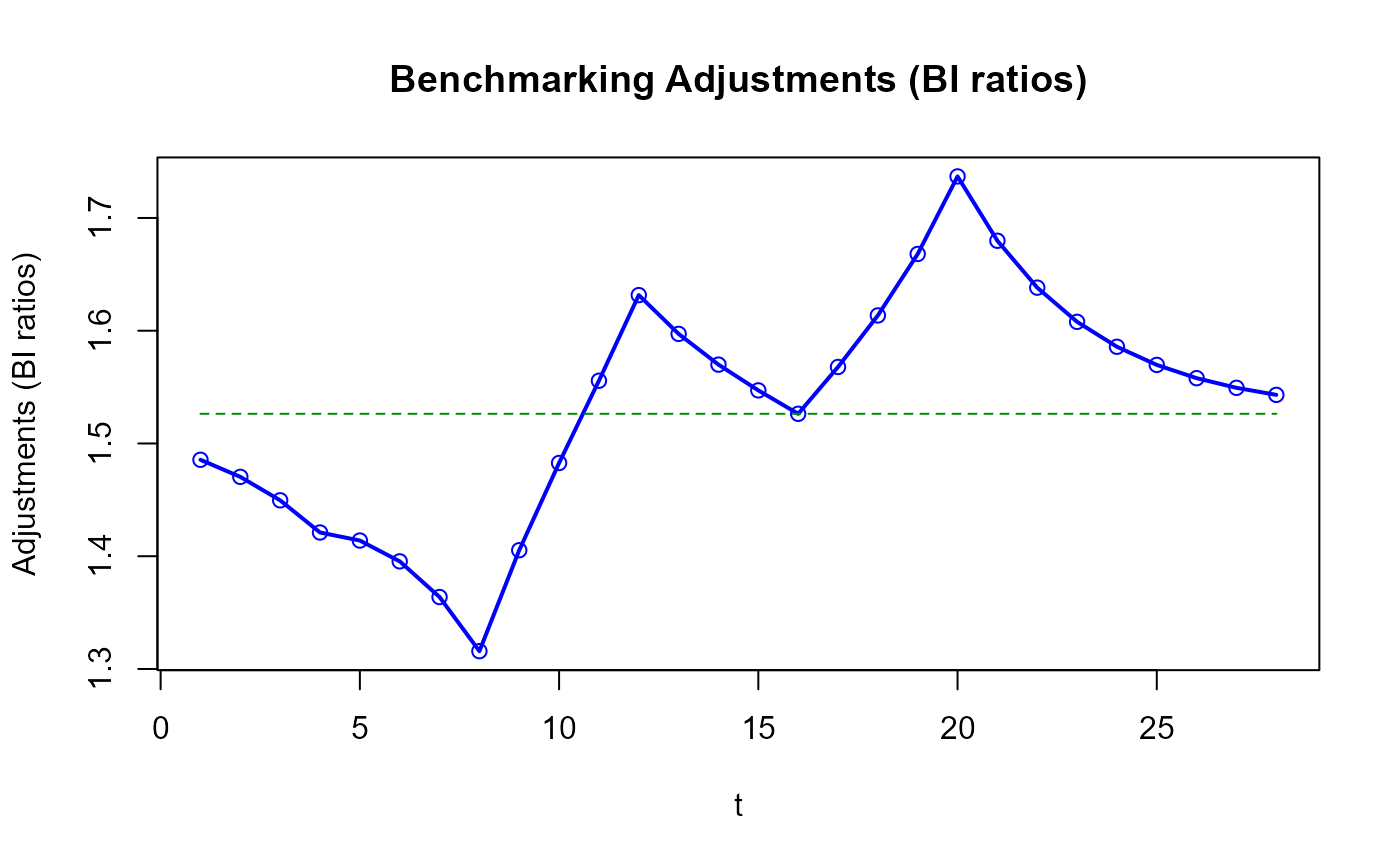
# `benchmarking()` adjustments (`out_PB`), without a legend
plot_benchAdj(PB_graphTable = out_PB$graphTable,
              legendPos = NULL)


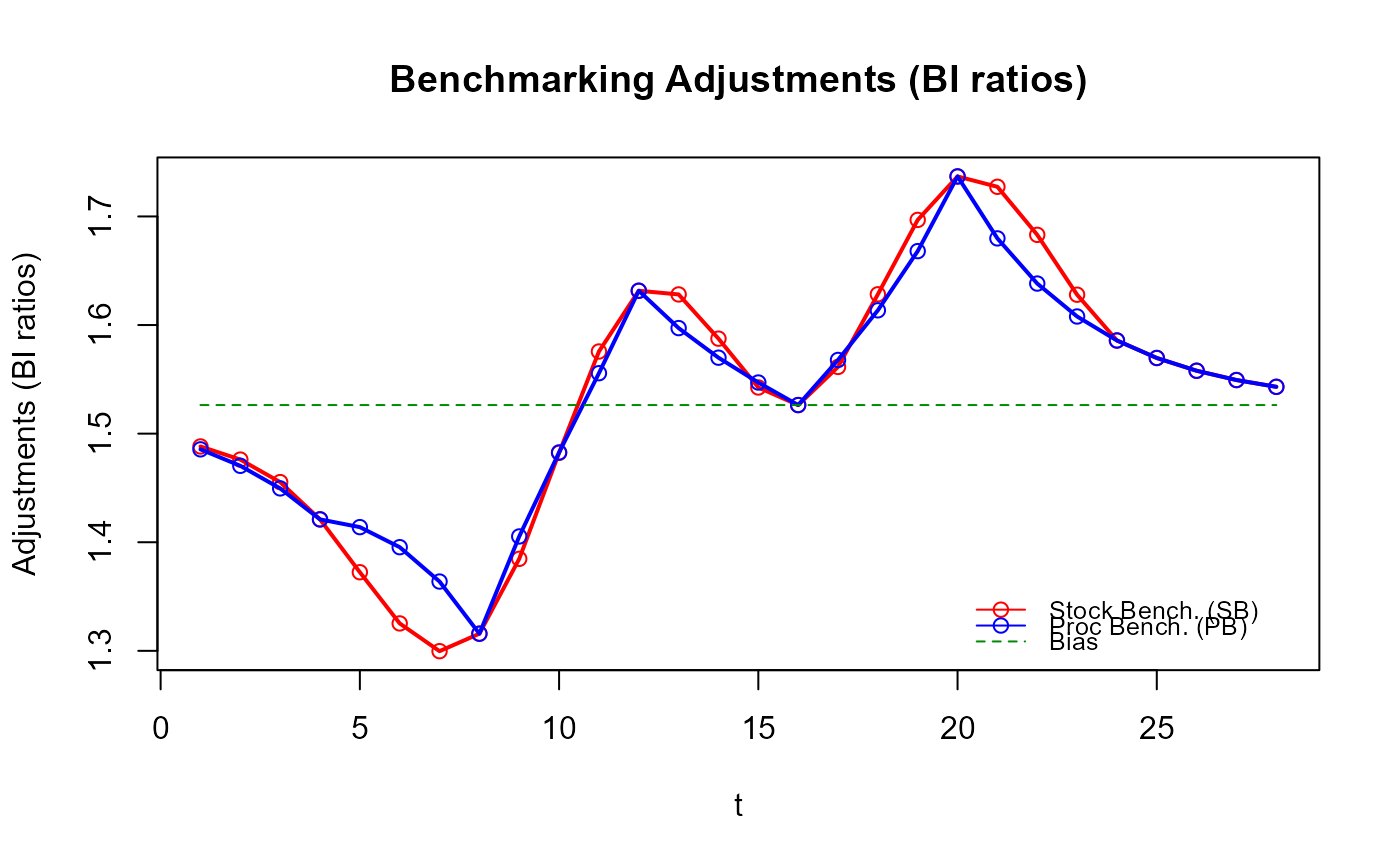
# Add the `stock_benchmarking()` (`out_SB`) adjustments, with a legend this time
plot_benchAdj(PB_graphTable = out_PB$graphTable,
              SB_graphTable = out_SB$graphTable)


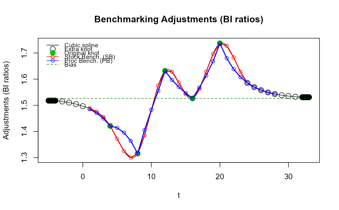
# Add the `stock_benchmarking()` cubic spline actually used to generate the adjustments
# (incl. the extra knots at both ends), with the legend located in the top-left corner
plot_benchAdj(PB_graphTable = out_PB$graphTable,
              SB_graphTable = out_SB$graphTable,
              SB_splineKnots = out_SB$splineKnots,
              legendPos = "topleft")



#######
# Simulate multiple series benchmarking (3 stock series)

qtr_mts <- ts.union(ser1 = qtr_ts, ser2 = qtr_ts * 100, ser3 = qtr_ts * 10)
ann_mts <- ts.union(ser1 = ann_ts, ser2 = ann_ts * 100, ser3 = ann_ts * 10)

# Using argument `allCols = TRUE` (identify stocks with column `varSeries`)
out_SB2 <- stock_benchmarking(
  ts_to_tsDF(qtr_mts),
  ts_to_bmkDF(ann_mts, discrete_flag = TRUE, alignment = "e", ind_frequency = 4),
  rho = 0.729, lambda = 1, biasOption = 3,
  allCols = TRUE,
  quiet = TRUE)
#> 
#> Benchmarking indicator series [ser1] with benchmarks [ser1]
#> -----------------------------------------------------------
#> 
#> Benchmarking indicator series [ser2] with benchmarks [ser2]
#> -----------------------------------------------------------
#> 
#> Benchmarking indicator series [ser3] with benchmarks [ser3]
#> -----------------------------------------------------------

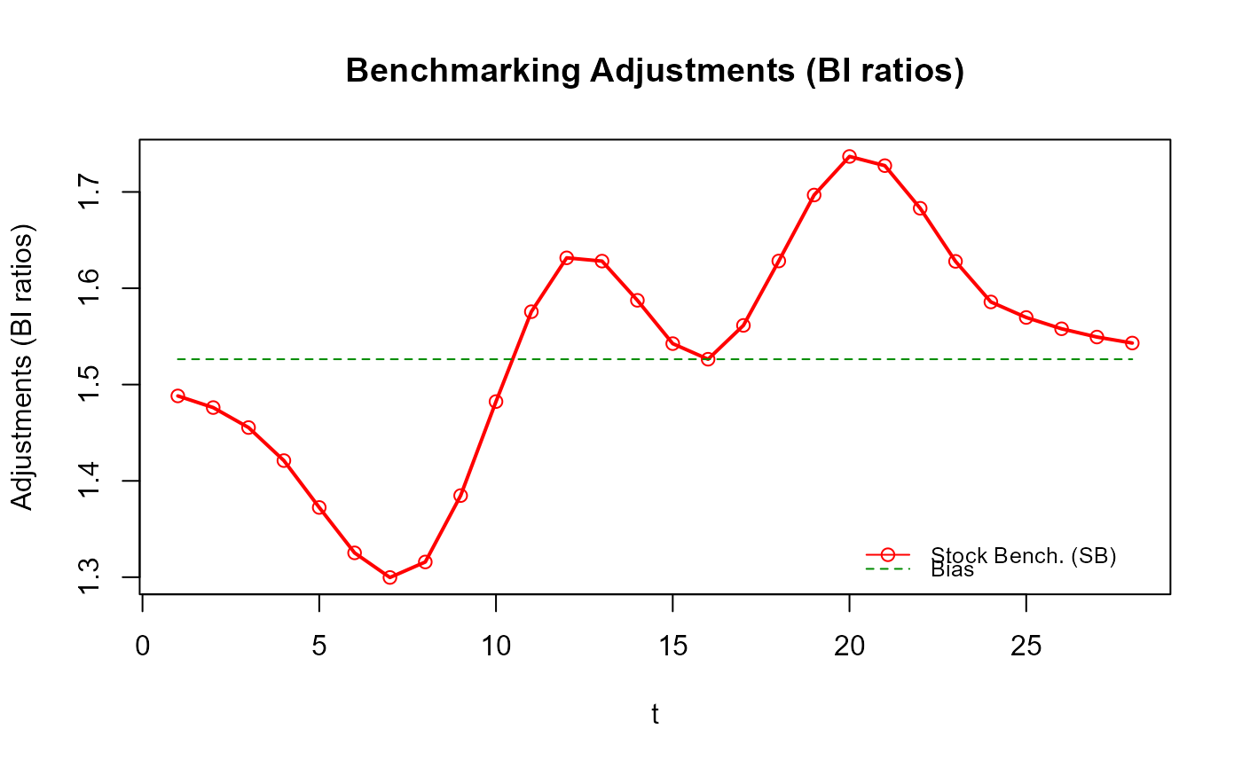
# Adjustments for 2nd stock (ser2)
plot_benchAdj(
  SB_graphTable = out_SB2$graphTable[out_SB2$graphTable$varSeries == "ser2", ])


# Using argument `by = "series"` (identify stocks with column `series`)
out_SB3 <- stock_benchmarking(
  stack_tsDF(ts_to_tsDF(qtr_mts)),
  stack_bmkDF(ts_to_bmkDF(
    ann_mts, discrete_flag = TRUE, alignment = "e", ind_frequency = 4)),
  rho = 0.729, lambda = 1, biasOption = 3,
  by = "series",
  quiet = TRUE)
#> 
#> Benchmarking by-group 1 (series=ser1)
#> =====================================
#> 
#> Benchmarking by-group 2 (series=ser2)
#> =====================================
#> 
#> Benchmarking by-group 3 (series=ser3)
#> =====================================

# Cubic spline for 3nd stock (ser3)
plot_benchAdj(
  SB_splineKnots = out_SB3$splineKnots[out_SB3$splineKnots$series == "ser3", ])