ReRun: Fast and Powerful Multimodal Data Visualization¶

Welcome to ReRun, your go-to SDK for visualizing multimodal data that dynamically evolves over time. Engineers and researchers in fields like computer vision and robotics leverage ReRun to verify, debug, and demonstrate their projects with unparalleled efficiency.

Key Highlights¶

• Open-Core Model: ReRun operates on an open-core model, ensuring that everything in this repository remains open source and free. In the future, ReRun will introduce a commercial product that builds upon the robust foundation of the core free project.

• Tailored for Individuals and Teams: The open source project caters to the needs of individual developers, while the upcoming commercial product will specifically address the requirements of teams involved in building and running computer vision and robotics products.

• Versatile and Cross-Platform: ReRun is an SDK and engine designed for visualizing and interacting with multimodal data streams. It's simple to integrate and get started with, usable from Python, Rust, and C++, and built in Rust for cross-platform compatibility and speed.

• Open Source: ReRun is committed to open source principles, dual-licensed under MIT and Apache 2.

Installation¶

To unleash the power of ReRun, install it in your JupyterLab environment with a simple command:

In [ ]:

%%capture
! pip install -U rerun-sdk

%%capture ! pip install -U rerun-sdk

Getting Started¶

For an optimal ReRun experience, it's recommended to use a Linux, Mac, or Windows desktop session instead of JupyterLab. Access the full ReRun viewer by running rr.spawn() in the following script from your terminal emulator:

import rerun as rr

rr.spawn()

However, if JupyterLab is your preferred environment, ReRun seamlessly operates within it. Refer to the official documentation for details on running ReRun within JupyterLab. The simplest JupyterLab example is to open ReRun using the memory_recording() and show() methods:

In [ ]:

import rerun as rr

rec = rr.memory_recording()
rec.show(width=1024, height=768)

import rerun as rr rec = rr.memory_recording() rec.show(width=1024, height=768)

3D Visualization: The Cube¶

Experience the simplicity of 3D visualization with ReRun by generating and plotting points in space:

In [ ]:

import rerun as rr
import numpy as np

rec = rr.memory_recording()

SIZE = 10

pos_grid = np.meshgrid(*[np.linspace(-10, 10, SIZE)]*3)
positions = np.vstack([d.reshape(-1) for d in pos_grid]).T

col_grid = np.meshgrid(*[np.linspace(0, 255, SIZE)]*3)
colors = np.vstack([c.reshape(-1) for c in col_grid]).astype(np.uint8).T

rr.log(
    "my_points",
    rr.Points3D(positions, colors=colors, radii=0.5)
)

rec.show(width=1024, height=768)

import rerun as rr import numpy as np rec = rr.memory_recording() SIZE = 10 pos_grid = np.meshgrid(*[np.linspace(-10, 10, SIZE)]*3) positions = np.vstack([d.reshape(-1) for d in pos_grid]).T col_grid = np.meshgrid(*[np.linspace(0, 255, SIZE)]*3) colors = np.vstack([c.reshape(-1) for c in col_grid]).astype(np.uint8).T rr.log( "my_points", rr.Points3D(positions, colors=colors, radii=0.5) ) rec.show(width=1024, height=768)

3D Visualization: The DNA¶

Explore a fascinating example of synthetic 3D data visualization in the shape of a double helix:

In [ ]:

from __future__ import annotations

import argparse
from math import tau

import numpy as np

import rerun as rr  # pip install rerun-sdk
from rerun.utilities import bounce_lerp, build_color_spiral

rec = rr.memory_recording()

rr.set_time_seconds("stable_time", 0)

NUM_POINTS = 100

# points and colors are both np.array((NUM_POINTS, 3))
points1, colors1 = build_color_spiral(NUM_POINTS)
points2, colors2 = build_color_spiral(NUM_POINTS, angular_offset=tau * 0.5)
rr.log("helix/structure/left", rr.Points3D(points1, colors=colors1, radii=0.08))
rr.log("helix/structure/right", rr.Points3D(points2, colors=colors2, radii=0.08))

rr.log("helix/structure/scaffolding", rr.LineStrips3D(np.stack((points1, points2), axis=1), colors=[128, 128, 128]))

time_offsets = np.random.rand(NUM_POINTS)
for i in range(400):
    time = i * 0.01
    rr.set_time_seconds("stable_time", time)

    times = np.repeat(time, NUM_POINTS) + time_offsets
    beads = [bounce_lerp(points1[n], points2[n], times[n]) for n in range(NUM_POINTS)]
    colors = [[int(bounce_lerp(80, 230, times[n] * 2))] for n in range(NUM_POINTS)]
    rr.log(
        "helix/structure/scaffolding/beads", rr.Points3D(beads, radii=0.06, colors=np.repeat(colors, 3, axis=-1))
    )

    rr.log(
        "helix/structure",
        rr.Transform3D(rotation=rr.RotationAxisAngle(axis=[0, 0, 1], radians=time / 4.0 * tau)),
    )

rec.show(width=1024, height=768)

from __future__ import annotations import argparse from math import tau import numpy as np import rerun as rr # pip install rerun-sdk from rerun.utilities import bounce_lerp, build_color_spiral rec = rr.memory_recording() rr.set_time_seconds("stable_time", 0) NUM_POINTS = 100 # points and colors are both np.array((NUM_POINTS, 3)) points1, colors1 = build_color_spiral(NUM_POINTS) points2, colors2 = build_color_spiral(NUM_POINTS, angular_offset=tau * 0.5) rr.log("helix/structure/left", rr.Points3D(points1, colors=colors1, radii=0.08)) rr.log("helix/structure/right", rr.Points3D(points2, colors=colors2, radii=0.08)) rr.log("helix/structure/scaffolding", rr.LineStrips3D(np.stack((points1, points2), axis=1), colors=[128, 128, 128])) time_offsets = np.random.rand(NUM_POINTS) for i in range(400): time = i * 0.01 rr.set_time_seconds("stable_time", time) times = np.repeat(time, NUM_POINTS) + time_offsets beads = [bounce_lerp(points1[n], points2[n], times[n]) for n in range(NUM_POINTS)] colors = [[int(bounce_lerp(80, 230, times[n] * 2))] for n in range(NUM_POINTS)] rr.log( "helix/structure/scaffolding/beads", rr.Points3D(beads, radii=0.06, colors=np.repeat(colors, 3, axis=-1)) ) rr.log( "helix/structure", rr.Transform3D(rotation=rr.RotationAxisAngle(axis=[0, 0, 1], radians=time / 4.0 * tau)), ) rec.show(width=1024, height=768)

Time-Series Data: Plots that Impress¶

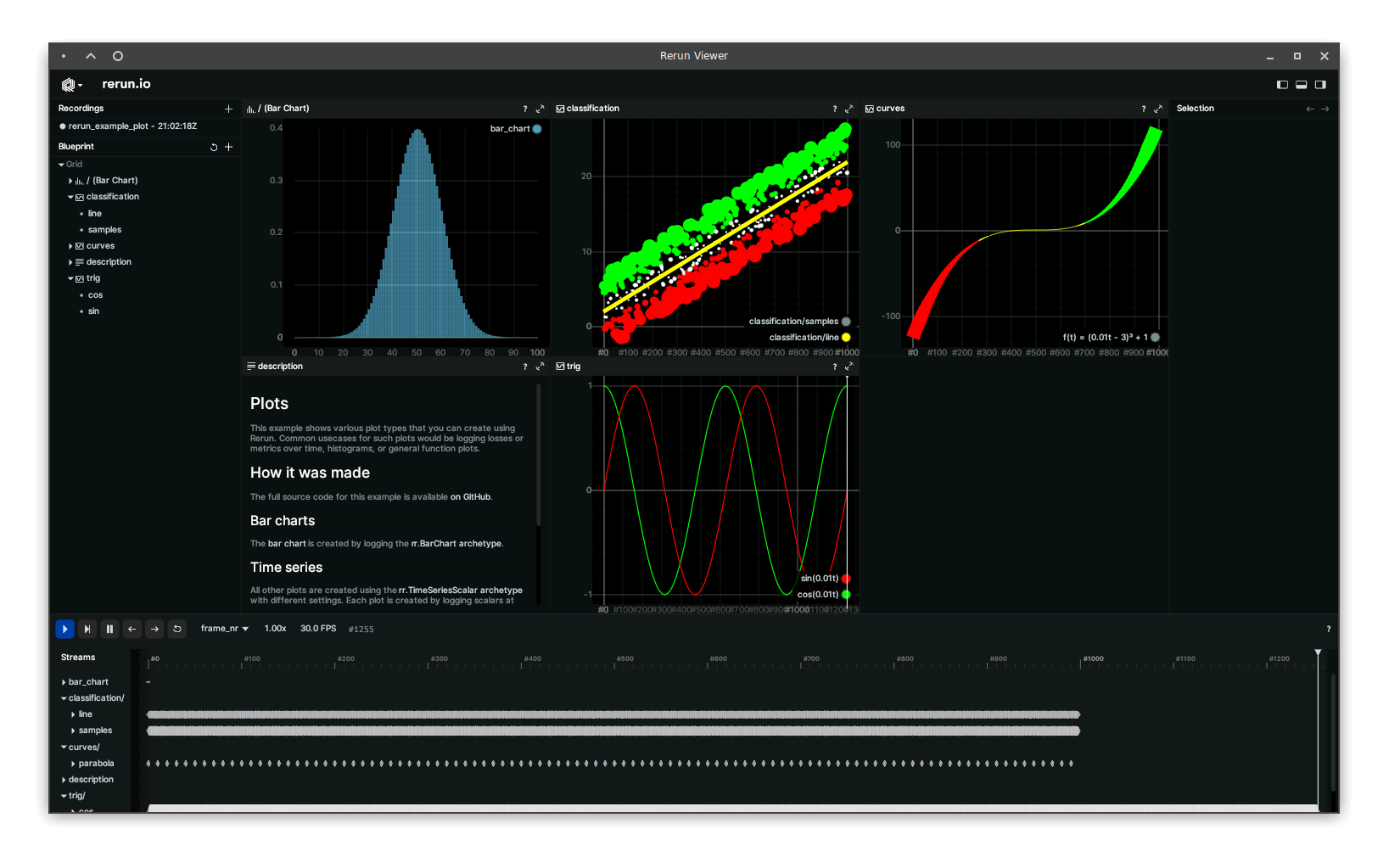
ReRun truly shines when visualizing multimodal time-series data. The following example demonstrates ReRun's prowess in displaying various plots corresponding to different readings on the same time-series data:

In [ ]:

from __future__ import annotations

import argparse
import random
from math import cos, sin, tau

import numpy as np
import rerun as rr  # pip install rerun-sdk

rec = rr.memory_recording()

def clamp(n, smallest, largest):  # type: ignore[no-untyped-def]
    return max(smallest, min(n, largest))


def log_bar_chart() -> None:
    rr.set_time_sequence("frame_nr", 0)
    # Log a gauss bell as a bar chart
    mean = 0
    std = 1
    variance = np.square(std)
    x = np.arange(-5, 5, 0.1)
    y = np.exp(-np.square(x - mean) / 2 * variance) / (np.sqrt(2 * np.pi * variance))
    rr.log("bar_chart", rr.BarChart(y))


def log_parabola() -> None:
    # Log a parabola as a time series
    for t in range(0, 1000, 10):
        rr.set_time_sequence("frame_nr", t)

        f_of_t = (t * 0.01 - 5) ** 3 + 1
        radius = clamp(abs(f_of_t) * 0.1, 0.5, 10.0)
        color = [255, 255, 0]
        if f_of_t < -10.0:
            color = [255, 0, 0]
        elif f_of_t > 10.0:
            color = [0, 255, 0]

        rr.log(
            "curves/parabola",
            rr.TimeSeriesScalar(
                f_of_t,
                label="f(t) = (0.01t - 3)³ + 1",
                radius=radius,
                color=color,
            ),
        )


def log_trig() -> None:
    # Log a time series
    for t in range(0, int(tau * 2 * 100.0)):
        rr.set_time_sequence("frame_nr", t)

        sin_of_t = sin(float(t) / 100.0)
        rr.log("trig/sin", rr.TimeSeriesScalar(sin_of_t, label="sin(0.01t)", color=[255, 0, 0]))

        cos_of_t = cos(float(t) / 100.0)
        rr.log("trig/cos", rr.TimeSeriesScalar(cos_of_t, label="cos(0.01t)", color=[0, 255, 0]))


def log_classification() -> None:
    # Log a time series
    for t in range(0, 1000, 2):
        rr.set_time_sequence("frame_nr", t)

        f_of_t = (2 * 0.01 * t) + 2
        color = [255, 255, 0]
        rr.log("classification/line", rr.TimeSeriesScalar(f_of_t, color=color, radius=3.0))

        g_of_t = f_of_t + random.uniform(-5.0, 5.0)
        if g_of_t < f_of_t - 1.5:
            color = [255, 0, 0]
        elif g_of_t > f_of_t + 1.5:
            color = [0, 255, 0]
        else:
            color = [255, 255, 255]
        radius = abs(g_of_t - f_of_t)
        rr.log("classification/samples", rr.TimeSeriesScalar(g_of_t, color=color, scattered=True, radius=radius))


log_bar_chart()
log_parabola()
log_trig()
log_classification()

rec.show(width=1024, height=768)

from __future__ import annotations import argparse import random from math import cos, sin, tau import numpy as np import rerun as rr # pip install rerun-sdk rec = rr.memory_recording() def clamp(n, smallest, largest): # type: ignore[no-untyped-def] return max(smallest, min(n, largest)) def log_bar_chart() -> None: rr.set_time_sequence("frame_nr", 0) # Log a gauss bell as a bar chart mean = 0 std = 1 variance = np.square(std) x = np.arange(-5, 5, 0.1) y = np.exp(-np.square(x - mean) / 2 * variance) / (np.sqrt(2 * np.pi * variance)) rr.log("bar_chart", rr.BarChart(y)) def log_parabola() -> None: # Log a parabola as a time series for t in range(0, 1000, 10): rr.set_time_sequence("frame_nr", t) f_of_t = (t * 0.01 - 5) ** 3 + 1 radius = clamp(abs(f_of_t) * 0.1, 0.5, 10.0) color = [255, 255, 0] if f_of_t < -10.0: color = [255, 0, 0] elif f_of_t > 10.0: color = [0, 255, 0] rr.log( "curves/parabola", rr.TimeSeriesScalar( f_of_t, label="f(t) = (0.01t - 3)³ + 1", radius=radius, color=color, ), ) def log_trig() -> None: # Log a time series for t in range(0, int(tau * 2 * 100.0)): rr.set_time_sequence("frame_nr", t) sin_of_t = sin(float(t) / 100.0) rr.log("trig/sin", rr.TimeSeriesScalar(sin_of_t, label="sin(0.01t)", color=[255, 0, 0])) cos_of_t = cos(float(t) / 100.0) rr.log("trig/cos", rr.TimeSeriesScalar(cos_of_t, label="cos(0.01t)", color=[0, 255, 0])) def log_classification() -> None: # Log a time series for t in range(0, 1000, 2): rr.set_time_sequence("frame_nr", t) f_of_t = (2 * 0.01 * t) + 2 color = [255, 255, 0] rr.log("classification/line", rr.TimeSeriesScalar(f_of_t, color=color, radius=3.0)) g_of_t = f_of_t + random.uniform(-5.0, 5.0) if g_of_t < f_of_t - 1.5: color = [255, 0, 0] elif g_of_t > f_of_t + 1.5: color = [0, 255, 0] else: color = [255, 255, 255] radius = abs(g_of_t - f_of_t) rr.log("classification/samples", rr.TimeSeriesScalar(g_of_t, color=color, scattered=True, radius=radius)) log_bar_chart() log_parabola() log_trig() log_classification() rec.show(width=1024, height=768)

Dive Deeper¶

For an in-depth understanding of ReRun and its capabilities, refer to the official ReRun Python Quickstart.

Now, armed with ReRun, embark on a journey of unparalleled data visualization and exploration. Happy coding!